|
We may often need to analyse data on filtered range. There may be requirement to count the cells, or sum the cells or find the maximum value of the cells or so on... In such situation only using the FUNCTIONs simply like SUM, MAX etc.. will not work. However if we use the function with their name like 3(for non blank cells i;e COUNTA) or 9(for summing the filtered range i;e SUM) or others as per actual requirement which are in built and available in excel, with SUBTOTAL function then it works perfectly. 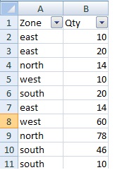 For your clear understanding please refer the above table. The table contains of different zone name and respective quantity field. Suppose if we want obtain total quantity of "east" zone then we need to use name of SUM function (which is 9) using the name range or reference with SUBTOTAL. Let filter the zone for "east". 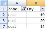 The function to be used like =SUBTOTAL(9,B2:B7) and the result will be appear 44. Here using simple SUM will give the result as 88.It is very useful where the filtered data is huge.
0 Comments
If you don't have any ready made software to generate form 16 for AY 2016-17, you can use this excel based application. It is suitable for small organisation. You may use this application to generate Form 16 for 100 employees. Before start read the instructions carefully and go ahead. While making data entry plese use TAB KEY to navigate in next cells. Please select PAN of the respective employee and also metnion the age group while generating Form 16.
In "citehr.com" one forum member had following issue: Aejaz.K Started The Discussion: Hi, I Have Excel Sheet Containing The Passport Details Such As Issue & Expiry. I Would Like Set Reminder Before The Expiry Date. I Have Been Trying On My Own But Couldn\'T Get The Desired Result. Need Your Help Thanks In Advance" http://www.citehr.com/391303-passport-expiry-reminder-excel-xls-download.html The above issue simply can be sorted out with the function of IF and Conditional Formatting. Find attached herewith the excel file. User only need to put Expiry Date in corresponding cells relating to Passport and Entry Visa Column ( column J and N). The function will automatically calculate Expiry Status. If the status is expired then respective row range will be highlighted with Red Color
Maintaining records of Student's Fee collection and tracking the same is a vital work in any school. In case of small schools often they do not use any software and mainly maintain the records on manually. Therefore to find any information like student wise, date wise etc may appear time consuming for the concerned person of that school. However using excel, one can maintain the aforesaid record very smartly. To give you the flavor of excel application, here I have designed a reporting format on Fee Collection, which mainly capture student wise collection status in any particular date as well enable to summarize class wise collection status at any given time period. Please download the file. Read the Help section, clear dummy records, key in your records and generate Report accordingly.
Have you ever tried VLOOKUP function to match multiple criteria? At least I had the idea of using INDEX and MATCH function to search Multiple criteria and use VLOOKUP for single criteria. Recently I have learned that to search on multiple criteria VLOOKUP function with a combination of CHOOSE can be used effectively. The formula would be like =VLOOKUP(Criteria1&Criteria2...,CHOOSE({1,2},Criteria Range1&Criteria Range2...,Lookup Range),2,0) press CTRL+SHIFT+ENTER key. Still have doubts? Ok, let refer the following example: 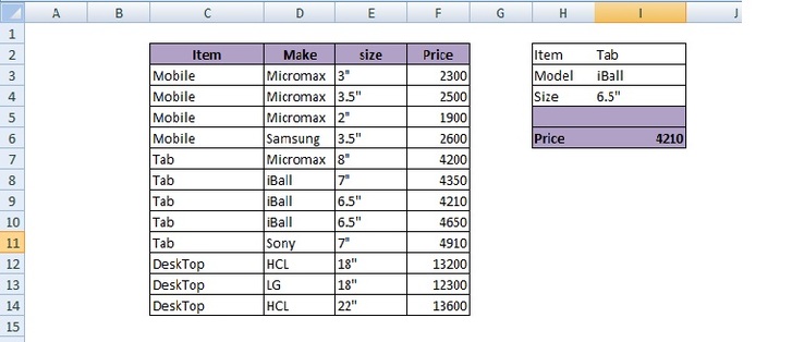 Suppose you want to get the price of any item with certain make and size. For example you wish to find the price of Tab having size 6.5" which is made by iball at cell no I6. To do the same you need to write the function as
=VLOOKUP(I2&I3&I4,CHOOSE({1,2},C3:C14&D3:D14&E3:E14,F3:F14),2,0) and press CTRL+SHIFT+ENTER You can try it using your own criteria and notice the amazing power of VLOOKUP One user in a forum of Excel Help asked solution for the following: "I have an Excel worksheet in which I log my flight hours. There are two primary columns: Column A is the date of my flight and column B is the number of hours flown for that particular flight. There can be multiple flights per day, so multiple rows per day. I am continually adding rows to the flight log. I need a way to calculate the number of hours flown over the last X days, where X could be 183 (6 months) or 365 (12 months). Any guidance would be much appreciated. —Forrest Voss " Answer: Using SUMIFS function the above can be solved. Please see the attached file.
There is some one who has asked about how to conditional format based on the following criteria: Subrata.Tatamotor "I Have A Spreadsheet With Two Different Value For Example Column A Column B Column C 100 100 200 150 80 100 I Want If Column A Data Match With The Col B Data Automatically Colour Formatting Done With Diff Value If Not Match Diff Colour Appearing On The Col C" Solution: Subrata, you can try the following to format the column on conditions. Based on your query, I think you are trying to colour the format of column C(from cell C1:C3) on satisfying following conditions: 1) If cell value of Column A matches with cell value of Column B ( here I have marked the cell in Yellow colour in respective cell in column C) 2) If cell value in Column A does not match with column B ( here I have marked the cell in Red colour in respective cell in column C) 3) More over I have considered here also,that if there is no value in cell A and B column i mean blank cell then the difference will be appear as blank in column C and the respective cell will be remain with no color. So to do the conditional format as mentioned above please go through below steps: Go to Home Menu--> Select conditional format-->Select "Use a formula to determine which cells to format" Put the format as per following: =AND($A1=$B1,NOT(ISBLANK($A1)),NOT(ISBLANK($B1))) Click "Format" button and select the "Fill" color. Here I have selected "yellow" color. Press "Ok". In applies to area, put the formula as =$C$1:$C$3 Press New Rule. In formula are put the formula as:=$A1<>$B1. Select Format and repeat the above step. In here I have selected "red" color. Press "OK" . In applies to area, put the formula as =$C$1:$C$3 and click on "Apply" button. =$C$1:$C$3 For calculating difference of Column A & B put the formula in Cell C1 as follwing: =IF(AND(ISBLANK(A1),ISBLANK(B1)),"",A1-B1) Copy the above formula in C2:C3 The above formula will calculate the difference only if there is no cell blank, other wise cell values in Column C will remain blank with no color format. Try it..
Please find herewith a very easy method how to create a Dynamic Chart using Drop down list. In here I have considered simple data and chart format to enable any one understand the step by step procedure how to make a Dynamic chart.
Often there is requirement to show numeric value in thousand unit. Without using formula you can covert the numeric value in thousand unit. Please go through the attached file.
|
Archives
November 2016
|
||||||||||||||||

